
Interactive Tutorial
Excel Pivot Table Conditional Formatting
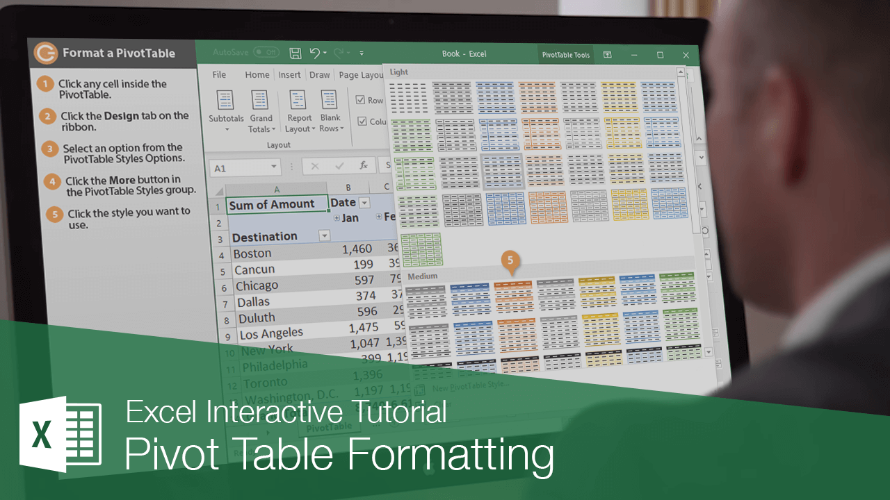
Apply Conditional Formatting to Pivot Tables in Excel to Highlight Key Trends and Data Patterns
-
Learn by Doing
-
LMS Ready
-
Earn Certificates

Try this Course with a Free Trial
After creating a PivotTable, you may want to enhance the look of it using styles. By default, the column headings, grand total row, and any filters have a light shading applied to the cells based on the workbook’s theme colors. However, if you don’t like these, there are a variety of other styles to choose from.
Work with Style Options
You can select PivotTable style options that allow you to adjust the format for part of a PivotTable. For example, you can apply special formatting to row headers or make the columns banded.
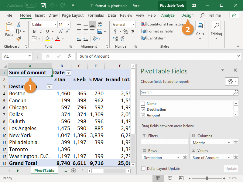
- Click any cell in the PivotTable.
- Click the Design tab.
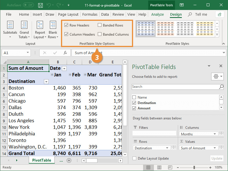
- Select an option from the PivotTable Style Options group.
- Row/Column Headers: Displays special formatting for the first row or column of the PivotTable.
- Banded Rows/Columns: Applies a different format to alternate rows or columns.
Apply a Built-In Style
Excel also has a gallery of built-in styles you can choose from to quickly format a PivotTable.
- On the Design tab, select an option in the Styles gallery.
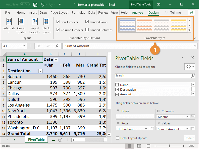
The PivotTable Styles group will show a few table styles, but to see the rest, you’ll need to expand the gallery.
The style is applied to the table, changing the borders, shading, and colors.
To remove a Table Style, select Clear from the More PivotTable Styles menu.