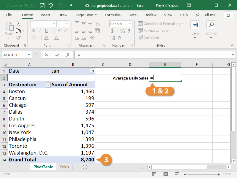
The GETPIVOTDATA function is used to extract data from your PivotTable. You place the function in a cell outside of the PivotTable, and it uses data within the table to perform a calculation. The syntax for the GETPIVOTDATA function looks like this: =GETPIVOTDATA (data_field, pivot_table, [field1, item1], ...). You fill in the function with the following information:
- data_field: The name of the field in the PivotTable you want to query.
- pivot_table: Any cell located in the PivotTable.
- field1, item1 (Optional): The field or item you wish to reference.
- Click in a cell outside the PivotTable where you want to add the function.
- Type the = sign.
- Click the cell in the PivotTable that contains the data you want to extract.
As soon as you type = and click within the PivotTable, the GETPIVOTDATA function is automatically added.
- (Optional) Expand the function to include additional calculations.
The advantage of using the GETPIVOTDATA function instead of a cell reference is that it records data to ensure the correct value is returned, even if the location of the referenced cell changes when the data in a PivotTable is updated.
If you happen to be using cube functions as part of your Excel workbooks, note the GETPIVOTDATA function has almost all of the expressions you'll need for your cube functions. You can paste these GETPIVOTDATA values into your cube functions to save time and simplify the process.

