Pivot Table in Excel

When faced with a worksheet packed full of data, with many columns and perhaps hundreds or thousands of rows, making sense of it all can be a daunting task. PivotTables help you pull out just the data you need to quickly make informed decisions. They are very flexible, easy to adjust, and can be created and modified with just a few clicks. Don’t worry if PivotTables are confusing at first, they will make a lot more sense once you start working with them.

Your data should be neatly organized into rows and columns without any blank rows or columns.

• Your data should be neatly organized into rows and columns without any blank rows or columns.
• Each column should have the same data type. For example, you shouldn’t have a column of prices where some cells have the currency format applied and some have the accounting format applied
• PivotTables can be created using a cell range or an existing table.

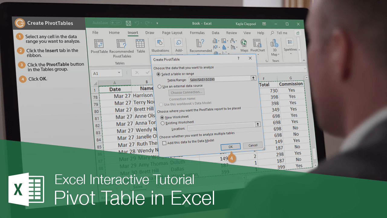
Create a PivotTable

1. Select any cell in the data range you want to analyze.
2. Click the Insert tab on the ribbon.
3. Click the PivotTable button in the Tables group.

   The Create PivotTable dialog box opens. Here, choose which data to analyze and where to place the PivotTable.

   If you’ve already clicked within a data range, the Table/Range field is populated. Verify the correct range is displayed.

   The data range doesn’t have to be in the current workbook. Select Use an external data source to select data outside the workbook.

4. Click OK.
   

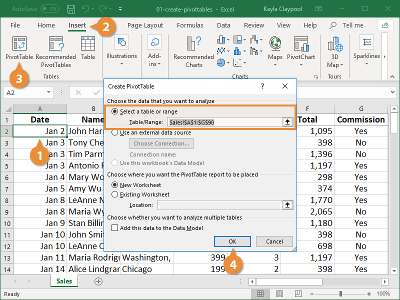
An empty PivotTable and task pane appear on a separate worksheet. Next you need to specify the fields you want to appear in your PivotTable.

Add PivotTable Fields

Once you’ve created your PivotTable, you have to specify the data you want to analyze. The PivotTable Fields pane appears at the right. Under the Search field you see a list of all the possible fields you can use in your PivotTable. These fields are the column headings from the original data source.

To make it a little easier to understand, let’s break it down. Say your original data set contains information for ticket sales and includes dates, destinations, prices, the number of sales, sales totals, sales agents, etc., but all you really need to know is how many tickets were sold each month for each destination. You can grab the Destination field and the Date field, add them as rows and columns in the PivotTable, and add a numeric sales field to the values area. The PivotTable will display a subset of the original data, but only include the values you really need to see.

1. Click and drag a field to the Rows area.
2. Click and drag a field to the Values area.
3. If desired, click and drag a field to the Columns area.
   

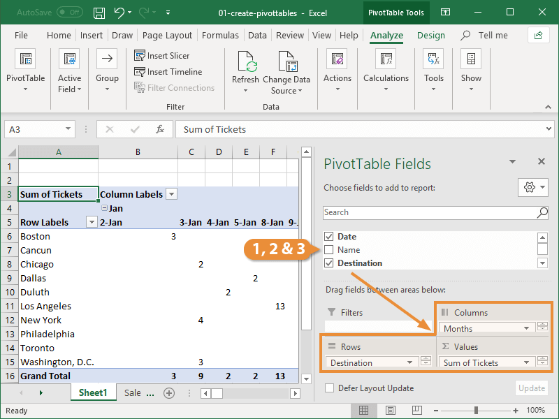
   If you want to filter the PivotTable, add an additional field to the Filters area.

The PivotTable updates to display the values for the fields you’ve added. The great thing about PivotTables is they are extremely flexible. If the table isn’t displaying the data like you want, just click and drag fields in and out of the Rows, Values, and Columns areas until the PivotTable represents the data correctly.