How to Add Axis Labels to a Chart in Excel

Adding elements like gridlines, labels, and data tables help viewers more easily identify what’s being presented.

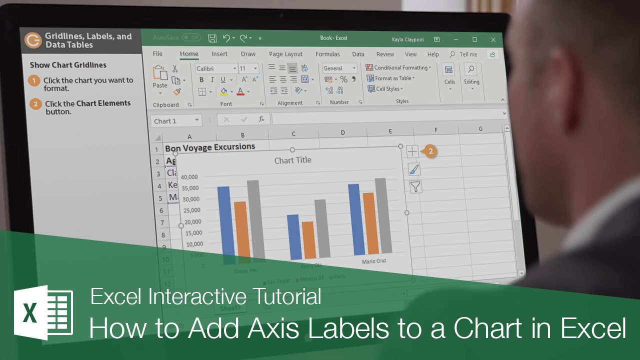
Show Chart Gridlines

Gridlines are the lines in the background of a chart that correspond to the values in the chart. In column and bar charts, gridlines make it easier to compare the values in the chart.

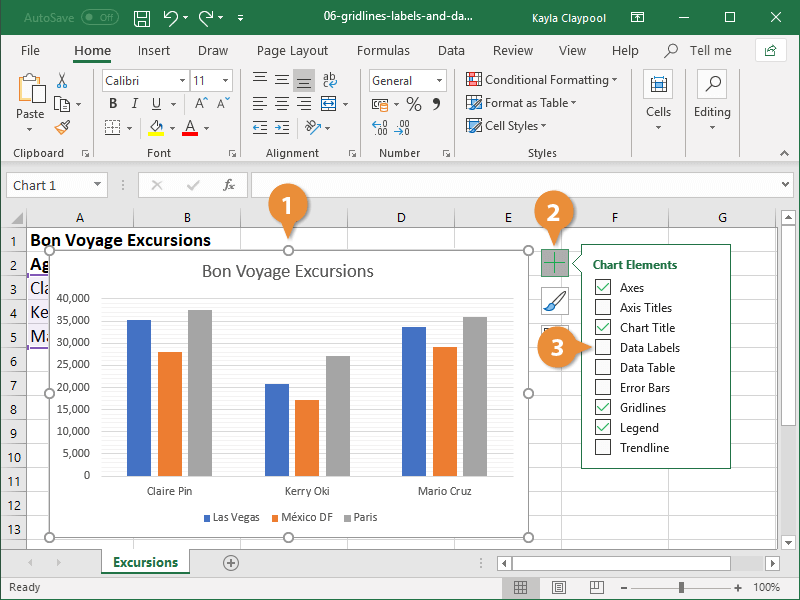
1. Select the chart you want to format.
2. Click the Chart Elements button.
3. Click the Gridlines list arrow.

   Be careful not to click the word Gridlines or all the gridlines will turn off, just hover over it until the list arrow appears.

4. Select the set of gridlines you want to show.
   

Add Data Labels

Use data labels to label the values of individual chart elements.

1. Select the chart.
2. Click the Chart Elements button.
3. Click the Data Labels check box.
   

   In the Chart Elements menu, click the Data Labels list arrow to change the position of the data labels.

Display a Data Table

A data table is a table that contains the data and headings from your worksheet that comprises the chart data.

1. Select the chart.
2. Click the Chart Elements button.
3. Click the Data Table check box.
   

   To edit the data table settings, hover over Data Table in the Chart Elements menu, click the list arrow, and select More Options.

A table with all the data represented in the chart is added below the chart’s plot area.