Excel Slicers

Slicers are a feature in Excel that provide an easy way to filter table data. They allow you to filter and re-filter your data quickly so it’s easy to find the exact information you need. Slicers work well when used with both tables and PivotTables.

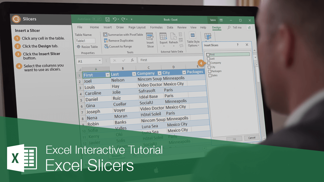
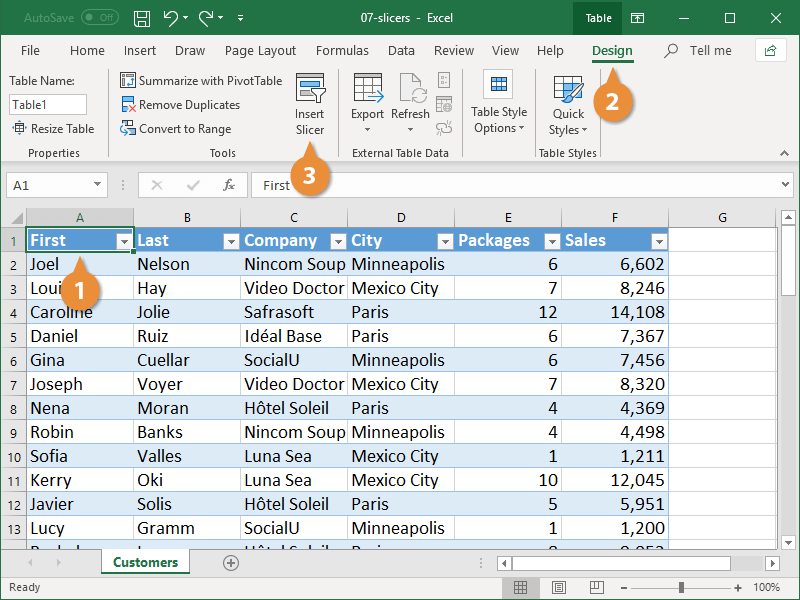
Insert a Slicer

1. Click any cell in the table.
2. Click the Design tab.
3. Click the Insert Slicer button.

   You can also click the Insert tab, then click Slicer.

   

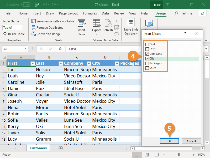
   The Insert Slicers dialog box appears. All the column headings in the table are listed here.

4. Select the columns you want to use as slicers.

   A separate slicer will be created for each column that’s selected.

5. Click OK.
   

The slicers appear in the worksheet. You can now move or resize them as needed.

Filter with a Slicer

After a slicer is created, it appears on the worksheet alongside the table. The slicers will be layered on top of one another if there is more than one, but they can easily be repositioned.

1. Select the values you want to include in the filter.
2. Hold down the Ctrl key to select multiple filters.
   

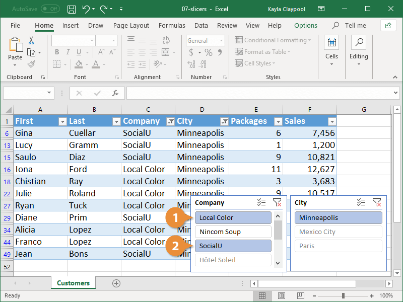
The table is filtered to show only the selected value(s).

While holding down the Ctrl key, simply click the value again to stop filtering the selected data.

Clear and Remove a Slicer

Before you delete a slicer from a worksheet, make sure you clear it. Deleting a slicer doesn’t clear the filter.

1. Click the Clear Filter button.

   All the filters are cleared, but the Slicer remains on the worksheet.

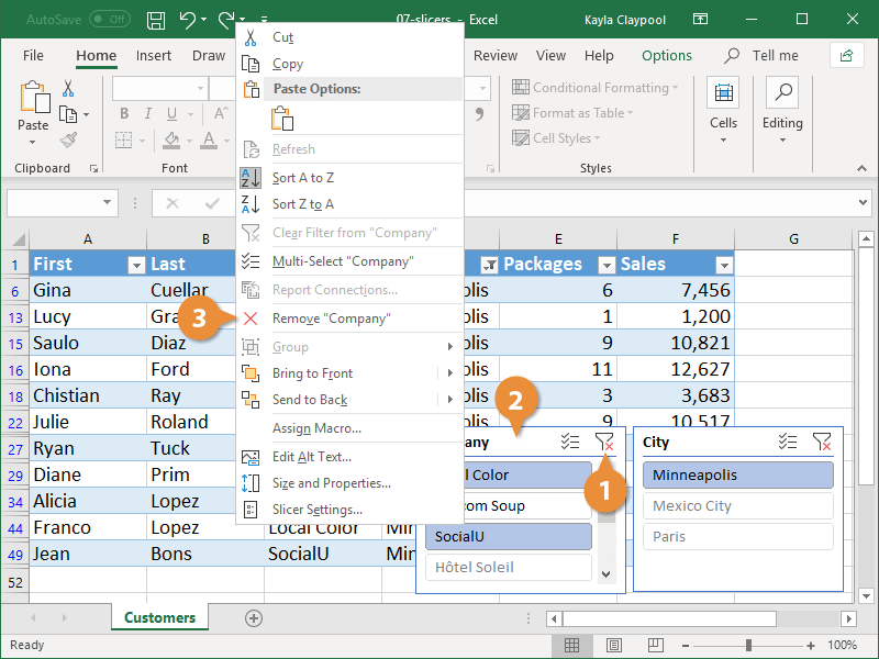
2. Right-click the slicer.
3. Select Remove “Filter name”.
   

   Click the slicer and press the Delete key.