Excel Conditional Formatting

Conditional formatting applies formats to cells only if a specified condition is true. For example, use conditional formatting to change cells with a sales value over $50,000 to have red, bold font. If the value of the cell changes and no longer meets the specified condition, the cell returns to its original formatting.

Apply Conditional Formatting

1. Select the cells you want to change.
2. Click the Cell Styles button on the Home tab.
   
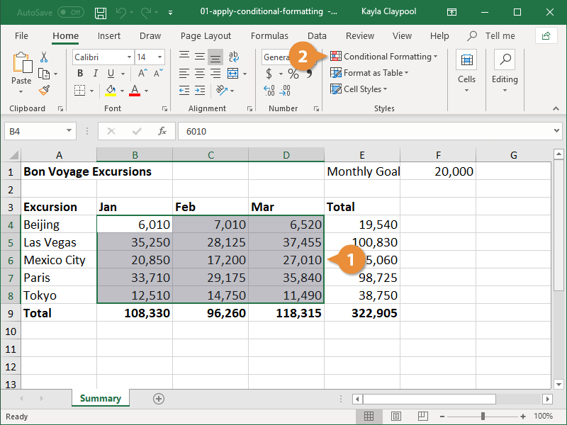
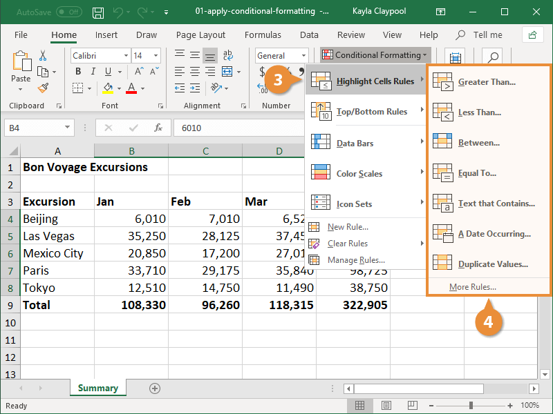
3. Select a conditional formatting category.
   • Highlight Cells Rules: Focus on general analysis. Preset conditions include: Greater Than; Less Than; Between; Equal To; Text That Contains; Date Occurring; Duplicate Values.
   • Top/Bottom Rules: Focus on the high and low values in the worksheet. Preset conditions include: Top 10 Items; Top 10%; Bottom 10 Items; Bottom 10%; Above Average; Below Average.
   • Data Bars: Colored bars that appear in the cells. The longer the bar, the higher the value in that cell.
   • Color Scales: Cells are shaded different color gradients depending on the relative value of each cell compared to other cells in the range
   • Icon Sets: Different shaped or colored icons appear in cells, based on each cell’s value. Select a conditional formatting rule.
4. Select a conditional formatting rule.
   
5. Specify the formatting to use for items that meet the conditional formatting criteria.
   

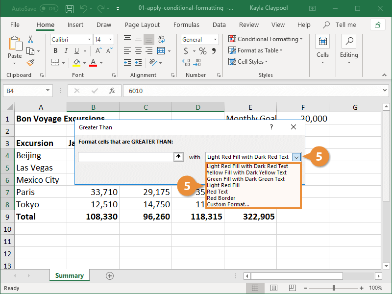
   The options you see in the dialog box will vary depending on the type of rule you selected.

6. Click OK.

Only the cells that meet the criteria are formatted.

Manage Conditional Formatting Rules

You can manage all aspects of conditional formatting—creating, editing, and deleting rules—in one place using the Rules Manager.

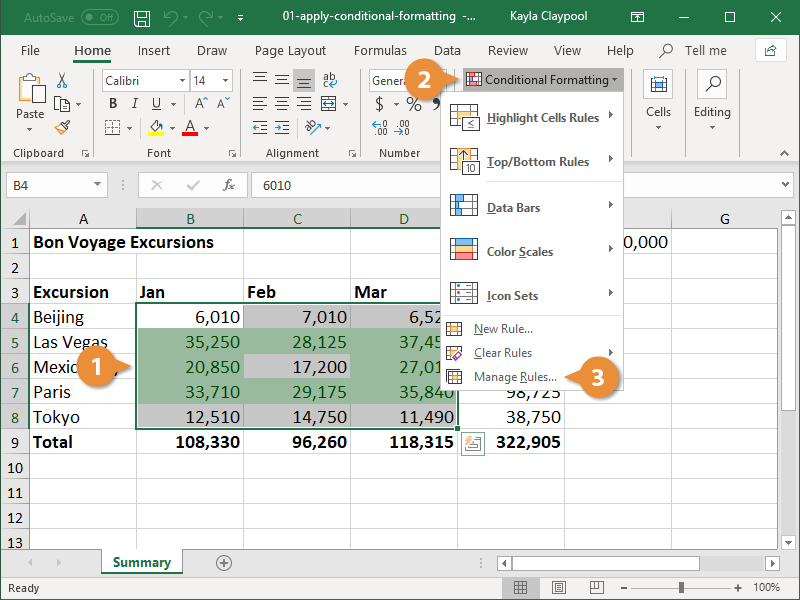
1. Select the cell range with the conditional formatting you want to manage.
2. Click the Conditional Formatting button on the Home tab.
3. Select Manage Rules.
   

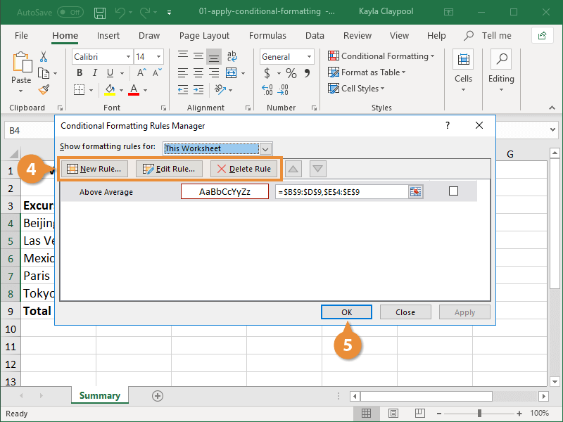
   The Conditional Formatting Rules Manager dialog box appears. The rules applied to the selected cells appear in the dialog box.

   Use these buttons to manage the rules:

   • New Rule: Create a brand new conditional formatting rule.
   • Edit Rule: Edit the selected formatting rule.
   • Delete Rule: Delete the selected rule from the worksheet.
4. Manage the formatting rules.
5. Click OK when you are finished.
   

Remove Conditional Formatting

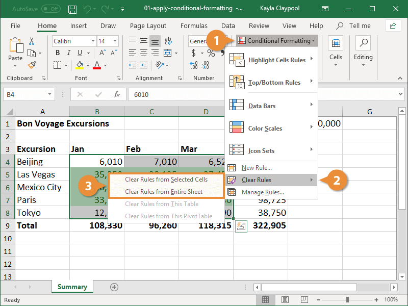
The Clear Rules command helps you remove conditional formatting rules from your worksheet.

1. Click the Conditional Formatting button on the Home tab.
2. Select Clear Rules.
3. Select a Clear Rules option:
   • Clear Rules from Selected Cells: Clears only the conditional formatting rules for the selected cell range.
   • Clear Rules from Entire Sheet: Clears all the conditional formatting rules in the worksheet.