Format Excel Chart Data

One way to emphasize chart data is to change the formatting of a specific piece of data or a data series so it stands out from the rest of the chart.

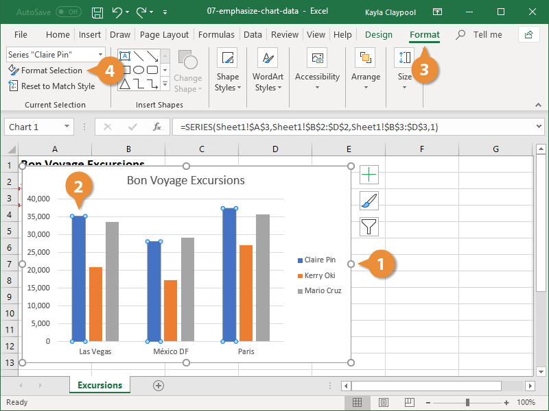
Change the Color of a Data Series

You can make a data series stand out by applying a different color to the series.

1. Select the chart you want to format.
2. Select the data series you want to format.
3. Click the Format tab.
4. Click Format Selection.
   

   Right-click a data series and select Format Data Series from the contextual menu.

   The formatting pane appears at the right.

5. Click the Fill & Line button.
6. Click Fill to expand the section.
7. Click the Fill Color button.
8. Select a color.
   

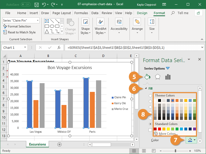
The formatting is applied to the entire data series.

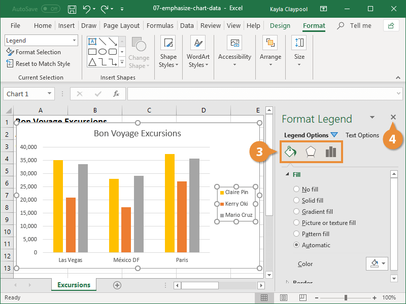
Format Other Chart Areas

You can also switch the chart element you want to format from right within the formatting panel.

1. Click the Series Options menu arrow.
2. Select a chart area to format.
   
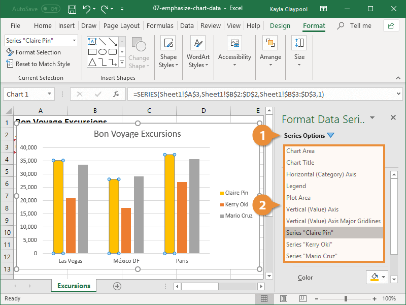
3. Select a type of format you want to apply.
4. Close the Format pane.