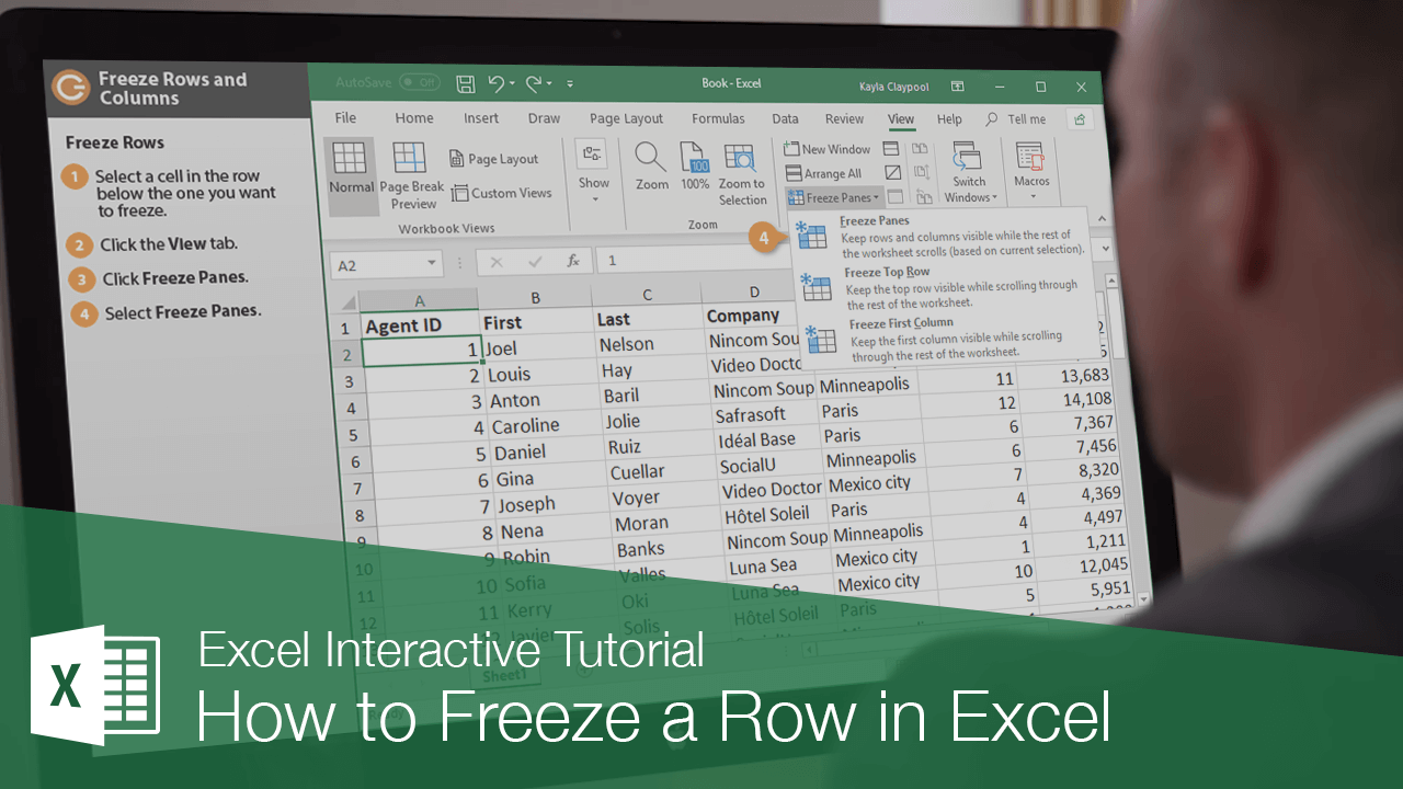
Interactive Tutorial
How to Freeze a Row in Excel
Learn How to Freeze Rows and Columns in Excel to Keep Headers Visible While Scrolling Through Data
-
Learn by Doing
-
LMS Ready
-
Earn Certificates

Try this Course with a Free Trial
When you're working in large spreadsheets, it can be hard to know what you're looking at once you scroll away from the header rows and columns. To fix this problem, you can freeze part of the worksheet so that even when you scroll, the headings are displayed.
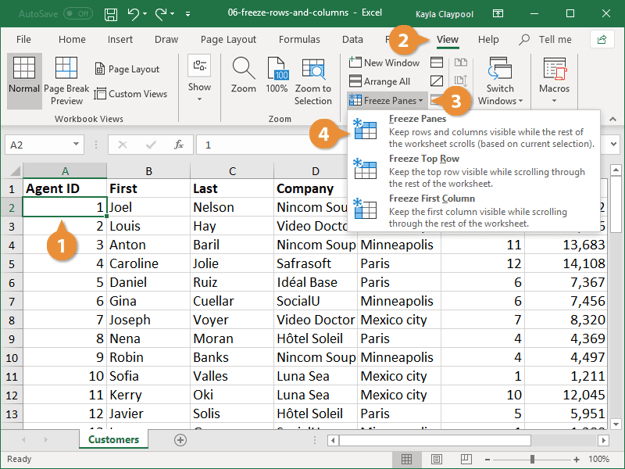
Freeze Rows
When you freeze panes, the rows above and columns to the left of the active cell are immobilized. In order to change the freeze point, you must unfreeze and freeze the cells again.
- Select a cell next to the row and/or column you want to freeze.
If you select a cell in the first column, only the rows above it will freeze (no columns). If you select a cell in the first row, only the columns to the left will freeze (no rows).
- Click the View tab.
- Click the Freeze Panes button.
- Select Freeze Panes.
- Scroll to verify the cells are frozen.
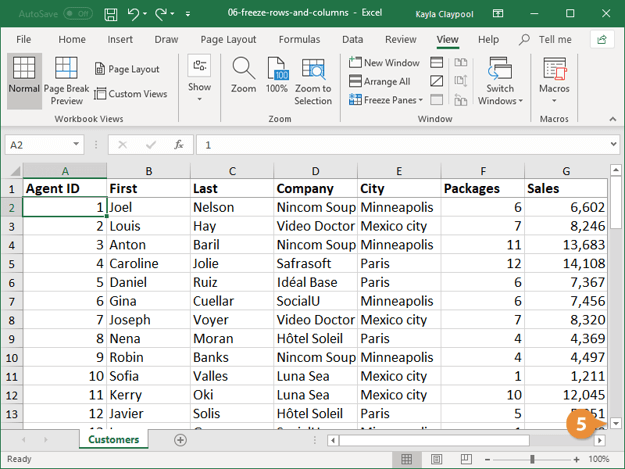
The frozen cells are visible no matter how far you scroll.
Freeze the First Row or Column
When you freeze only the first row or column, it doesn’t matter which cell is selected when the freeze is applied.
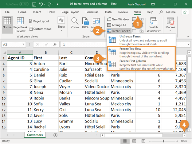
- Click the View tab.
- Ciick the Freeze Panes button.
- Select Freeze Top Row or Freeze First Column.
- Freeze Top Row Keeps the top row visible while scrolling through the worksheet.
- Freeze First Column Keeps the first column visible while scrolling through the worksheet.
- Scroll in the worksheet to verify the freeze is applied.
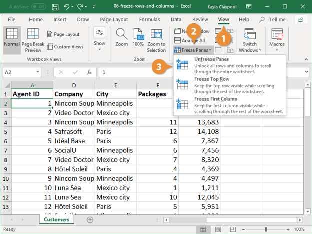
Unfreeze Panes
If you no longer need the cells in a spreadsheet to be frozen, you can unfreeze them at any time.
- Click the View tab.
- Click the Freeze Panes button.
- Select Unfreeze Panes.