
Interactive Tutorial
Index Match Excel
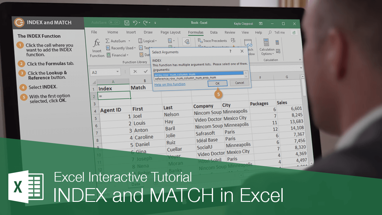
Master the INDEX and MATCH Functions in Excel to Create Dynamic and Accurate Data Lookups
-
Learn by Doing
-
LMS Ready
-
Earn Certificates

Try this Course with a Free Trial
While the INDEX and MATCH functions aren't overly powerful when used independently, together they allow you to return a cell value based on its vertical and horizontal position.
The INDEX Function
When used alone, the INDEX function returns a value at the intersection of a row and column you specify. For example, you can have Excel return the value at the intersection of row 2 and column 3.
The syntax for the INDEX function is fairly basic: =INDEX(array, row_num, [column_num]).
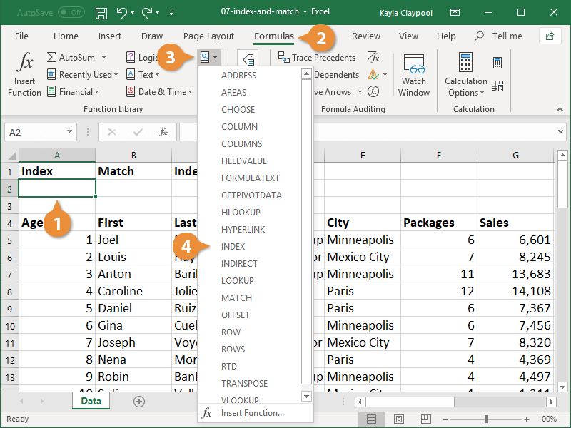
- Click in the cell where you want to add the INDEX function.
- Click the Formulas tab.
- Click the Lookup & Reference button in the Function Library group.
- Select INDEX.
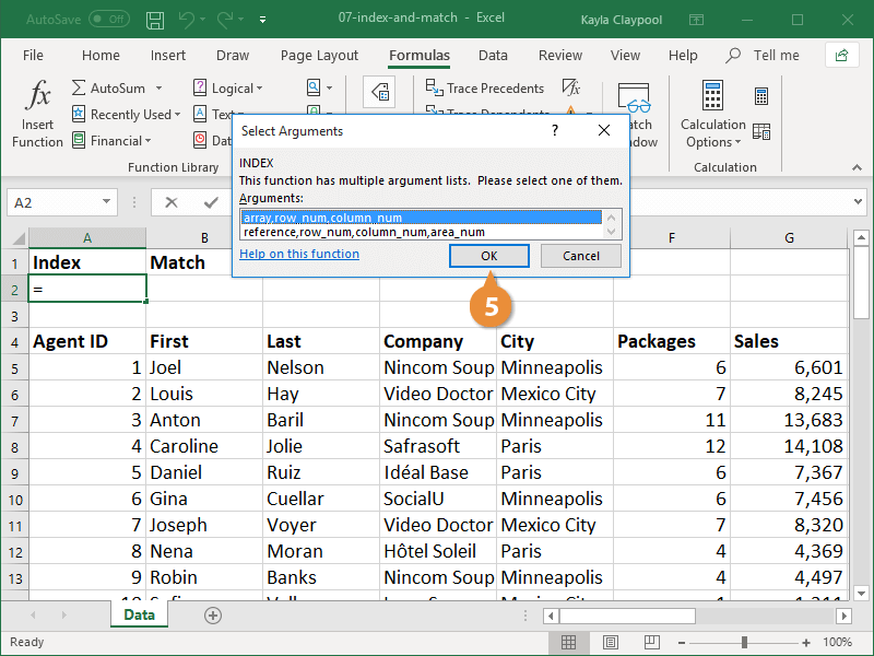
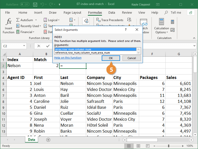
The Select Arguments dialog box appears. The INDEX function allows you to choose from two different sets of arguments.
- Array: Returns the actual value at the intersection of the row and column you specify.
- Reference: Returns the cell reference at the intersection of the row and column you specify.
- Select the array argument and click OK.
The Function Arguments dialog box displays where you’ll fill in the following arguments:
- Array: The range of cells in which you want to search.
- Row_num: The row in the array from which you want to return a value.
- Column_num: The column in the array from which you want to return a value. This is an optional argument.
- Enter the range of data you want to search in the Array field.
- Enter a new lookup value to search for in the first row of data.
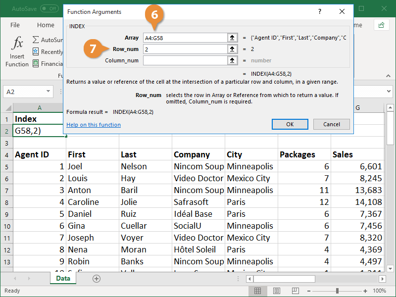
- Enter the row in the array you want search in the Row_num field.
The row and column you enter here refer to the row and column within the specified cell range, not the row and column number of the workbook.
There is a preview of the result located below the three argument fields. Check it to ensure the arguments are entered correctly and it's pulling out the correct value.
- Click OK.
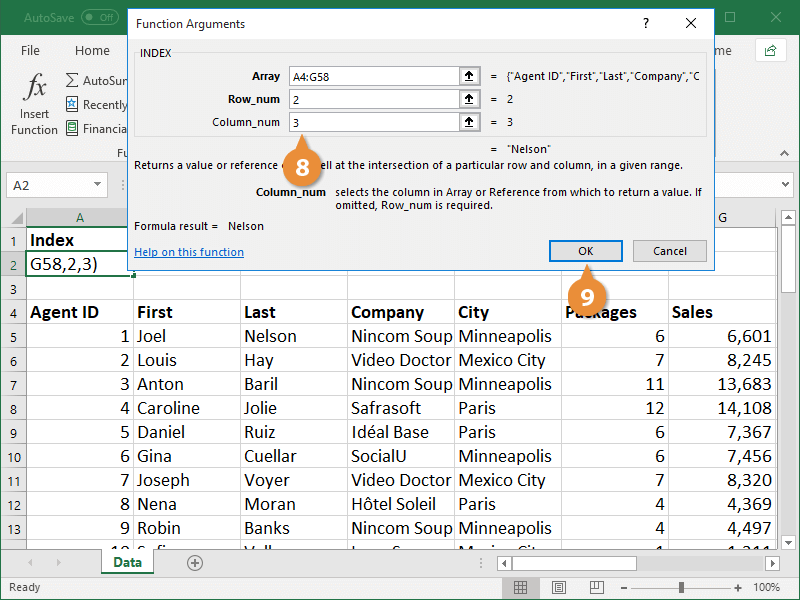
The INDEX function returns the value at the intersection of the row and column you specified.
The MATCH Function
When the MATCH function is used on its own, it searches for a value in a range of cells and returns the relative position of that value in the range. For example, you can have Excel look for the name Nelson in a column of last names and return the location in the column in which the name is found.
The syntax for the MATCH function looks like this: =MATCH (lookup_value, lookup_array, [match_type]).
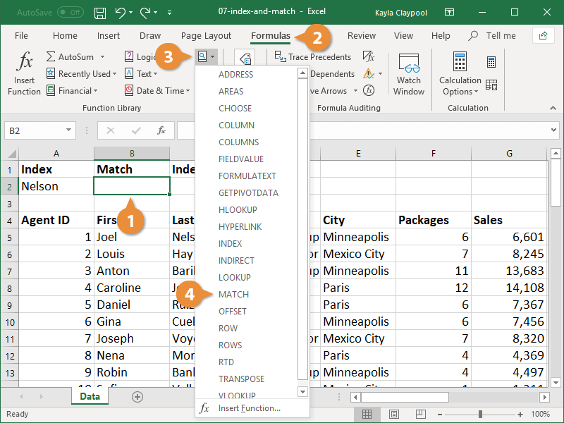
- Click in the cell where you want to add the MATCH function.
- Click the Formulas tab.
- Click the Lookup & Reference button in the Function Library group.
- Select MATCH.
The Function Arguments dialog box displays where you’ll fill in the following arguments:
- Lookup_value: The value in the cell range for which you want to find a cell reference.
- Lookup_array: A range of cells containing possible lookup values.
- Match_type: This is an optional argument. Enter 1, 0, or -1 to indicate which value to return. 1 or omitted finds the largest value that’s less than or equal to the lookup value, 0 returns an exact match, and -1 finds the smallest value that’s greater than or equal to the lookup value.
- Enter the value you want to search for in the Lookup_value field.
- Enter the value you want to search for in the Lookup_array field.
- Enter 0 in the Match_type field to search for an exact value.
- Click OK.
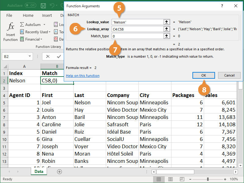
The MATCH function returns the location of the value in the cell range.
Combine the INDEX and MATCH Functions
When used together, the INDEX and MATCH functions combine to be a powerful force in Excel. After seeing how helpful these functions are, many people choose to use these instead of the VLOOKUP function.
Nesting the INDEX and MATCH functions allows you to look in a range of data and pull out a value at the intersection of any row and column. For example, you can start with the INDEX function and set a column of sales numbers as the array. Then within it, use the MATCH function to enter a name from a last name column. As a result, the formula will return the sales value for the name you specified.
While the VLOOKUP function can only look for a value in the first column of data to return an adjacent value, using the INDEX and MATCH functions together allows you to search any column and return a value in any row.
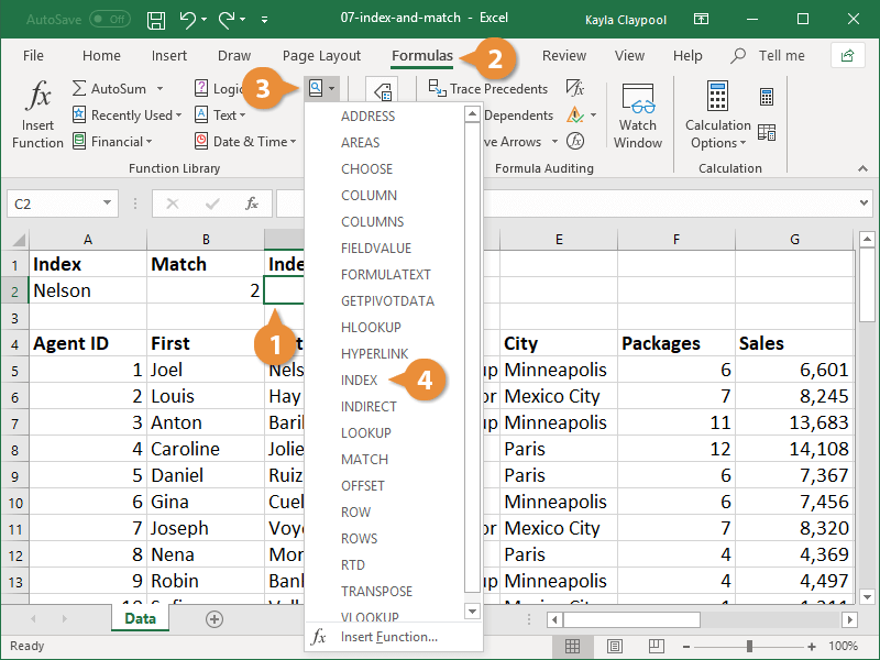
- Click the cell where you want to add the nested functions.
- Click the Formulas tab.
- Click the Lookup & Reference button in the Function Library group.
You will start with the INDEX function and nest the MATCH function within it.
- Select INDEX.
- Select the array argument option in the Select Arguments dialog box and click OK.
- Type the cell range you want to search within to locate a value.
This is often a single column of data, not a multi-column range.
- Enter the MATCH function in the Row_num field to specify the lookup value.
If the array is a single column, there is no need to add a value to the Column_num field, as there is only one column being searched.
- Click OK.
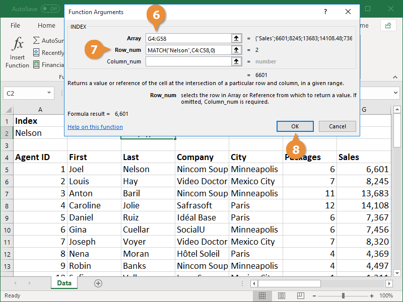
The nested function returns the value at the intersection of the array column and the value specified in the MATCH function.
If desired, you could take this a step further by modifying the lookup value of the MATCH function to find a different value in the INDEX array.