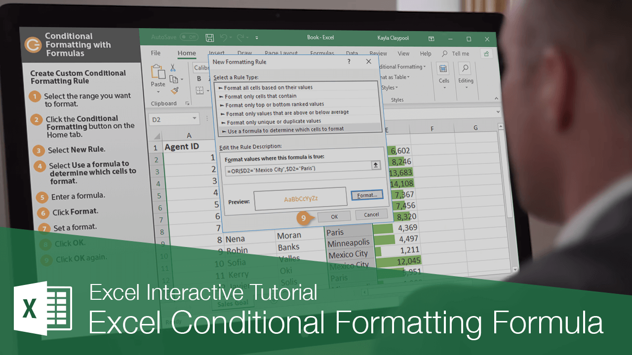
Excel Conditional Formatting Formula

Use Formulas with Conditional Formatting

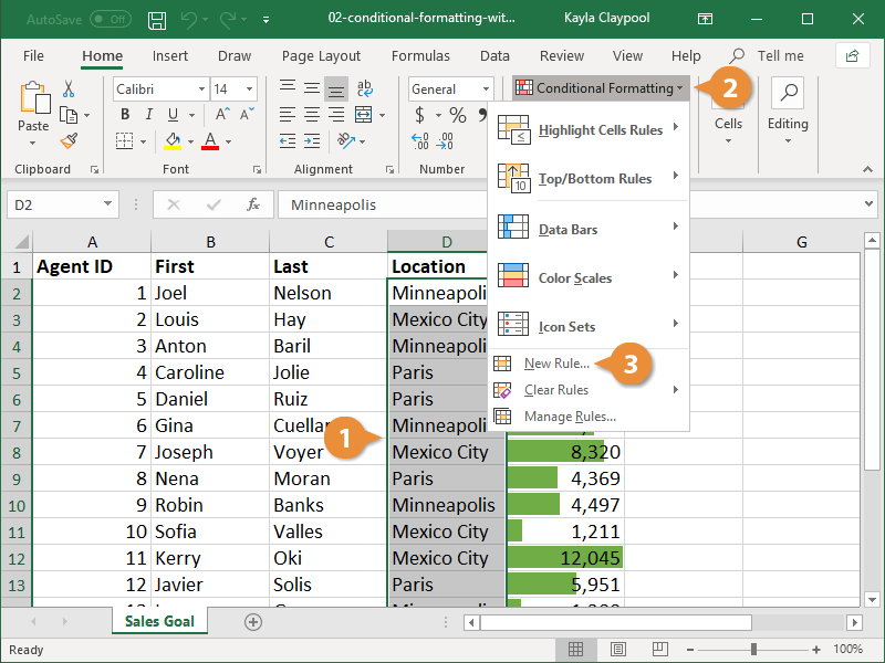
1. Select the range you want to format.
2. Click the Conditional Formatting button on the Home tab.
3. Select New Rule.
   

   The New Formatting Rule dialog box appears.

4. Select Use a formula to determine which cells to format.
5. Enter a formula in the Format values where this formula is true field.
6. Click the Format button.
7. In the Format Cells dialog box, specify the formatting you want to use and click OK.
   

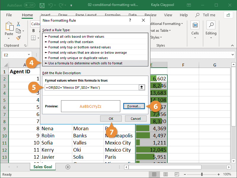
   A preview of the selected format displays at the bottom of the dialog box.

8. Click OK in the New Formatting Rule dialog box to save the custom rule.

The custom conditional formatting rule is saved.