How to Change Chart Data Range in Excel

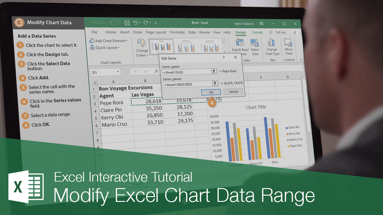
Once you see data in a chart, you may find there are some tweaks and changes that need to be made. Here are a few ways to change the data in your chart.

Add a Data Series

If you need to add additional data from the spreadsheet to the chart after it’s created, you can adjust the source data area.

1. Select the chart.
2. In the worksheet, click a sizing handle for the source data and drag it to include the additional data.
   

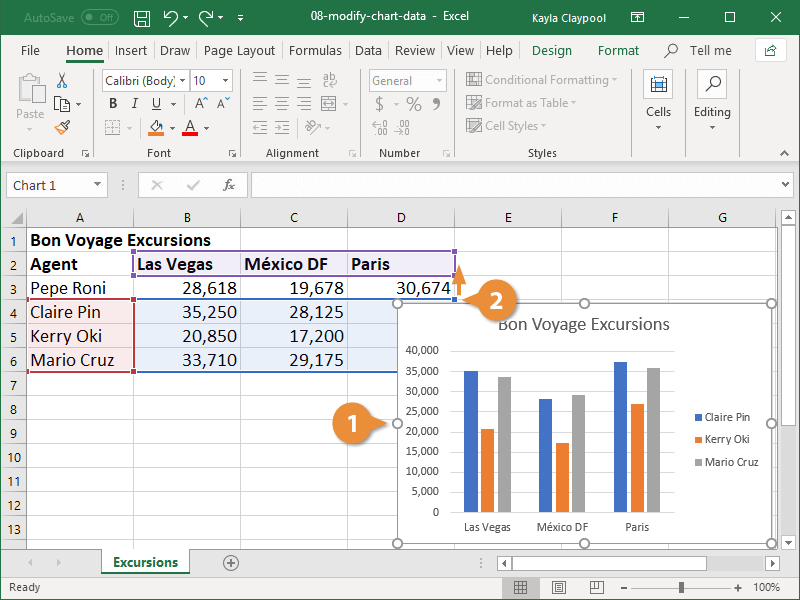
   The new data needs to be in cells adjacent to the existing chart data.

Rename a Data Series

Charts are not completely tied to the source data. You can change the name and values of a data series without changing the data in the worksheet.

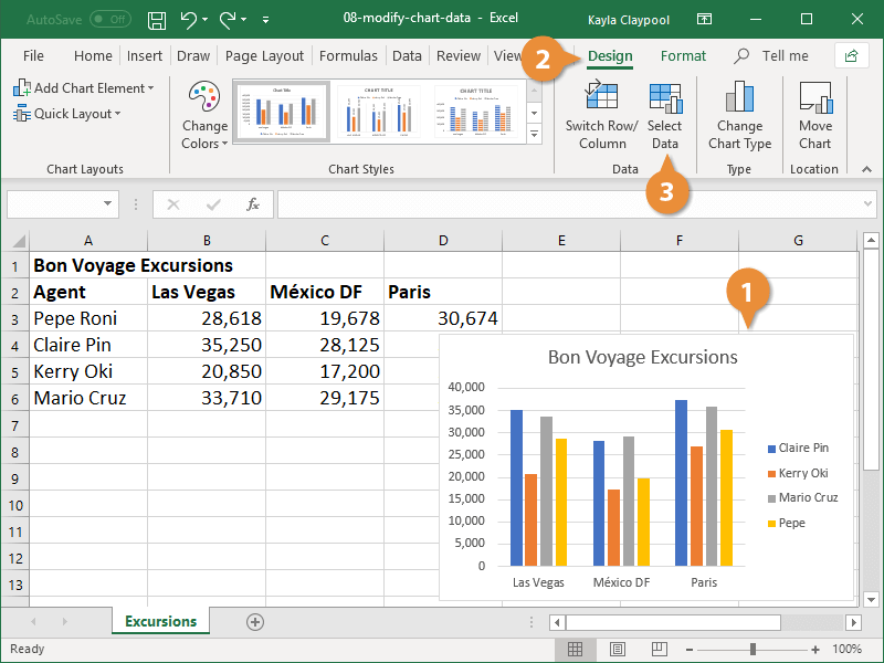
1. Select the chart
2. Click the Design tab.
3. Click the Select Data button.
   
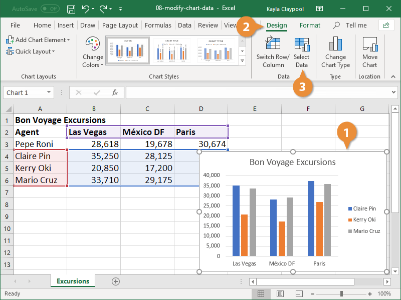
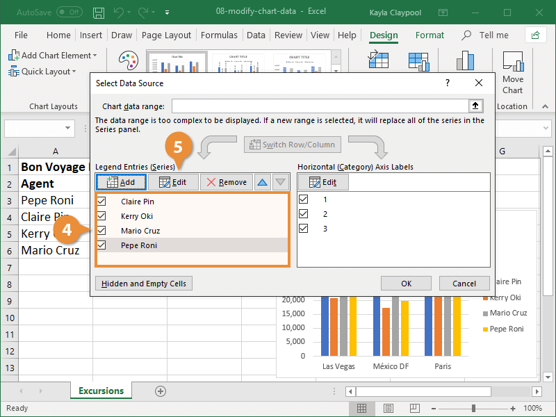
4. Select the series you want to change under Legend Entries (Series).
5. Click the Edit button.
   
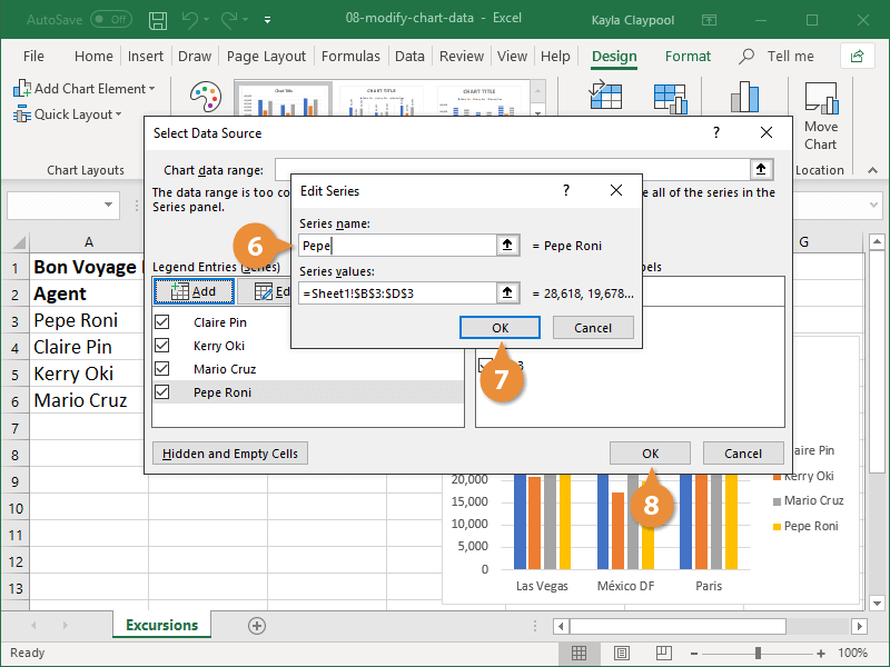
6. Type the label you want to use for the series in the Series name field.
7. Click OK.
8. Click OK again.
   

The name is updated in the chart, but the worksheet data remains unchanged.

Reorder a Data Series

You can also change the order of data in the chart without changing the order of the source data.

1. Select the chart
2. Click the Design tab.
3. Click the Select Data button.
   
4. From the Select Data Source dialog box, select the data series you want to move.
5. Click the Move Up or Move down button.
6. Click OK.
   

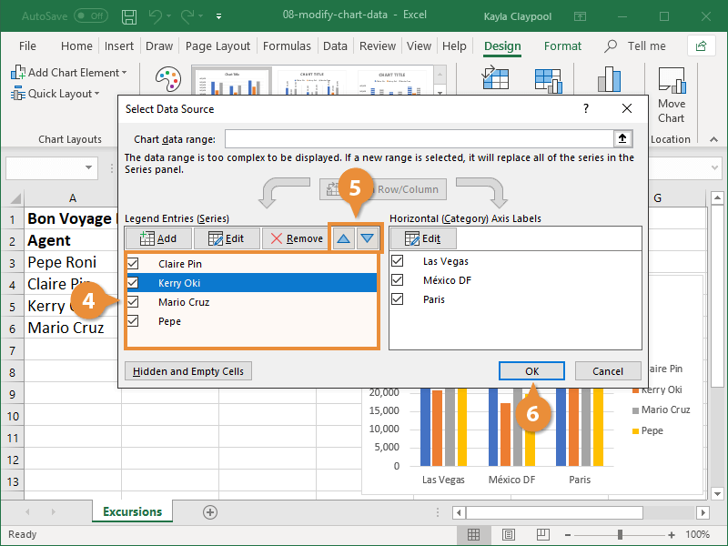
The chart is updated to display the new order of data, but the worksheet data remains unchanged.