Drill Down Excel Pivot Chart

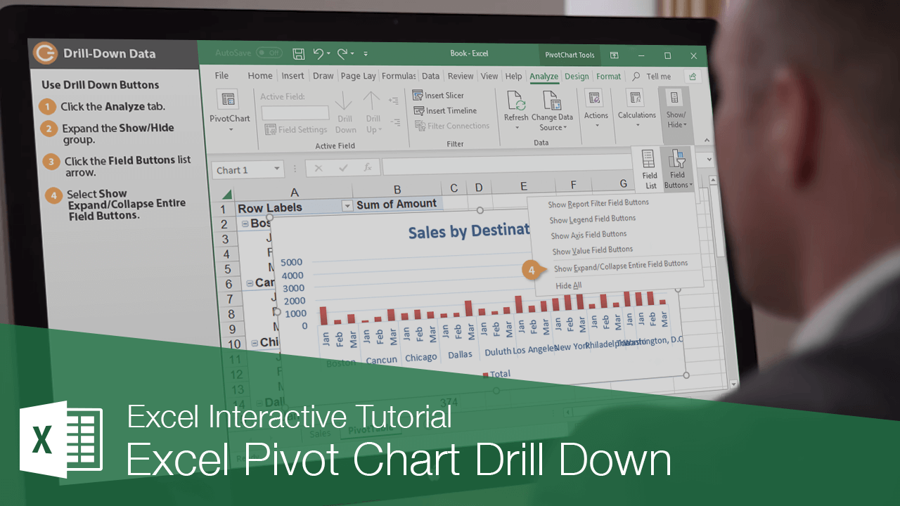
When you have more than one value on the X axis of a PivotChart, drilling down allows you to zoom in to or out of the data one level at a time.

Use Drill Down Buttons

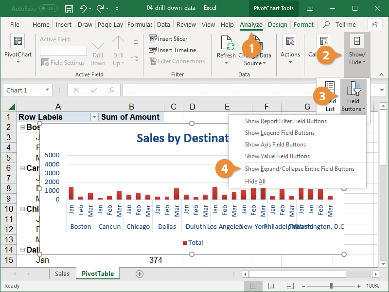
1. With the PivotChart selected, click the Analyze button.
2. Expand the Show/Hide group.
3. Click the Field Buttons list arrow.
4. Select Show Expand/Collapse Entire Field Buttons.
   

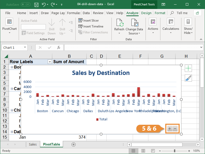
   The Drill Down buttons now appear at the bottom-right corner of the PivotChart.

   Even if the option is enabled, the Drill Down buttons will not appear on the PivotChart unless there is more than one value on the X axis.

5. Click the Collapse Entire Field (+) button to collapse the lowest level of data.

   The lowest level of data in the PivotChart is collapsed. Think of it as zooming out on the data.

6. Click the Expand Entire Field (+) button to expand the next level of data.
   

Drill Down into Specific Chart Data

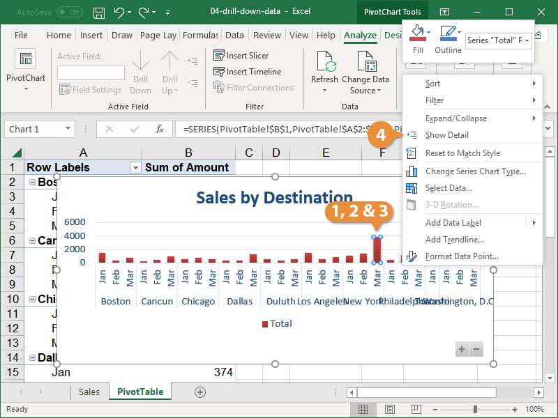
Often times, there will be a set of data in your PivotChart for which you’ll want to see more detailed information. For example, if the month of March had unusually high sales figures, you may want to see which team members helped contribute to the success. You can drill into a specific area of the chart to see what spreadsheet data contributes to that data point.

1. Select any series in the chart area.
2. Select the specific data set you want to drill down on.
3. Right-click the data set.
4. Select Show Detail in the menu.
   

All the data that makes up that specific data set is revealed on a separate worksheet. If, after you’ve reviewed the data, you no longer need this information, the sheet can be deleted.